By Pedro Hernández
On the official map, a piece of olive grove has an area and a land use. What the map does not say is how many trees stand inside it.
The public laser flight lets you measure that. It sweeps the ground with pulses of light and returns the height of the vegetation, crown by crown. That is the height model. Counting trees then means running a detector over it: a program that marks every local high point, one detection per mark.
In the Sierra Subbetica of Cordoba, Spain, the airborne laser scan of the 2024 public flight finds 130,668 crowns in the olive parcels of a 16 square kilometer frame, a square 4 kilometers on a side: at least 124.3 olive trees for every hectare the map draws, with a detector radius of 3.5 meters.
That is 1,743 parcels and 1,051.46 hectares: the olive parcels that fit whole inside the frame and cover at least 1,000 square meters. The parcel is the unit of the official map. SIGPAC maps Spanish farmland. It cuts each holding, meaning each farm as one owner works it, into parcels: one piece of ground, one land use, one outline, one area. Aid from the EU’s Common Agricultural Policy, the CAP, is paid on that map.
The “at least” is not a figure of speech. This method undercounts, and further down is why.
The frame has Carcabuey in its southwest quadrant and Priego de Cordoba about 6 kilometers to the east. The airborne laser scan, or LiDAR, flew over it in 2024. It left 9.7 measured points per square meter, nearly twice the minimum of five that this LiDAR product declares.
One more thing, measured in the previous article in this series and needed here: a hillside parcel has two surface areas. There is the one the map draws, which is flat, and the one you walk, which is always larger. In these same olive parcels there are 1,051.46 map hectares and 1,081.18 hectares of real ground, 2.83 percent more. Planting density changes depending on which of the two you divide by.
At least 124 olive trees per hectare, and the number that decides it
The height model measures whatever stands above the ground, plant or not, and that will matter further down. Across the 1,743 olive parcels the detector makes 130,668 detections, that is 130,668 crowns found, and the result depends on which of the two surface areas you divide by:
| Spread over | Olive trees per hectare |
|---|---|
| The 1,051.46 map hectares | 124.3 |
| The 1,081.18 hectares of real ground | 120.9 |
It is the opening fact seen from the other side: if the area rises 2.83 percent, trees per hectare fall 2.75 percent, because the same trees are spread over a larger base. The steeper the ground, the more it shows: in olive parcels between 30 and 40 percent slope the drop is 6.0 percent, and above 50 percent slope it is 15.4 percent, weighing each parcel by its hectares.
That figure rests on two chosen parameters, and publishing it without them would be publishing it badly. The first is the detector radius: the shortest distance two high points can be apart and still count as two crowns instead of one. The second is a height threshold, which leaves out anything not standing 1.2 meters above the ground. The radius is the one that rules.
| Detector radius | Olive trees per hectare |
|---|---|
| 2.0 m | 213.3 |
| 2.5 m | 172.4 |
| 3.0 m | 144.8 |
| 3.5 m | 124.2 |
| 4.0 m | 106.7 |
| 4.5 m | 91.1 |
We work at a radius of 3.5 meters. Two crowns closer together than that count as one, so the radius has to stay below the width of a mature crown. The table above covers every olive parcel in the frame, small ones included, and that is why its 3.5 meter row gives 124.2 instead of 124.3.
An inventory of the Andalusian olive grove publishes that width plot by plot for 35 olive groves in Jaen, worked out from aerial photos. It publishes no mean, and the mean of those 35 plots works out at 5.4 meters. The same table carries the widths held in the official plant health records, and those repeat exactly 4.0 meters in 26 of the 35 rows. A column that repeats one value that often tells you little about any single plot, so the width from the photo is the one that carries information here.
That width sets a ceiling. It does not pick a number: below the ceiling, both the 3.5 we use and the 4.5 in the last row fit. And these are mean widths per plot, not crowns measured one by one, so inside a plot there will be crowns narrower than its mean. The “at least” in the heading holds inside that choice, and that is why the figure travels with its radius attached.
The height threshold trims from below. Of the detections in the olive grove, 3.6 percent stand between 1.2 and 2 meters. That is a narrow band just above the threshold, and a young planting drops under 1.2 meters easily and goes uncounted.
Not one of the 296 detections reviewed sits on bare soil
We then went through them one by one, and that part can be redone with the same aerial photos. The review covered 296 detections on aerial photography from PNOA, the Spanish national aerial imagery program, at 25 centimeters per pixel, counting tree by tree. There were six windows, each 60 meters on a side and inside parcels over 0.8 hectares. Five were spread across very different slopes, at 3, 11, 30, 40 and 46 percent, and a sixth was picked at random. Not one detection falls on bare soil. Every one sits on a crown. That rules out one kind of failure, marking crowns where there are none, and leaves the other kind standing: failing to mark the ones that are there. Whether that crown belongs to an olive tree is a separate question, and it comes further down.

The failures the review did find are of the other kind. Some crowns go undetected, and they cluster where crowns touch and the height model merges them into a single high point. Where trees stand apart, between 92 and 97 percent are found. Where they merge, between 65 and 85 percent.
The limits of that check travel with it. It was done on screen and not in the field: nobody has counted an olive tree on the ground. The aerial photo of this area is from August to November 2022 and the laser scan is from 2024. And in dense olive grove, how many trees there are is ambiguous even by eye, because one olive tree can have several trunks that come out of the same root. What the check settles is the sign and the order of magnitude of the error, not a detection rate with decimals.
Why 124.3 is a lower limit and not a headcount
The sign of that error is the part most often left unsaid. The height threshold already trims from below. On top of it come three more failures, and the three do not pull the same way.
One takes trees out of the count: two olive trees whose crowns touch count as one. How much it takes out is what the review above has just measured. The other two add trees. An olive tree with several separated trunks can be counted twice. And the detector looks for height, not species. A holm oak, an almond tree or the roof of a farmhouse inside a parcel declared as olive grove enters the count as one more olive tree.
124.3 olive trees per hectare is a lower limit at that radius, and it is one because the three do not weigh the same. The one that takes trees out is measured, and it is large. The detector misses between 3 and 8 percent of the trees even where crowns stand apart, and between 15 and 35 percent where they merge. The two that add trees are not measured, but the detector itself puts a limit on each of them.
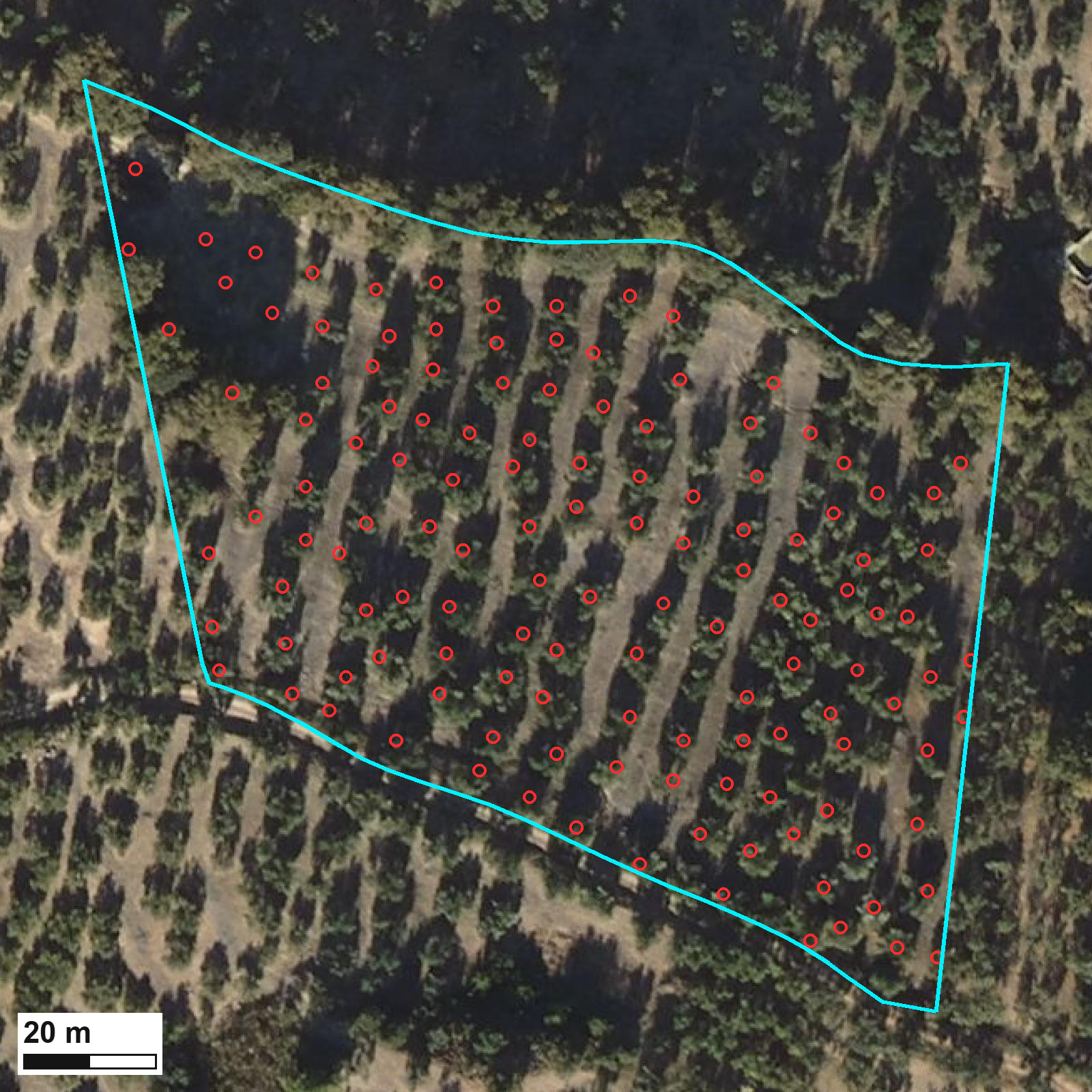
To count one olive tree twice, its trunks have to stand more than 3.5 meters apart. That is over a third of the local planting spacing, the distance the trees were set at, whose median here is 8.9 meters. As for the trees that are not olive trees, only the tall ones give themselves away. Of the 130,668 detections in the olive grove, 1,136 stand above 8 meters. That is 0.87 percent of the detections. In the parcel that opens this article it is three out of 133.
What stays unbounded is the almond tree the size of an olive tree, which gives itself away by nothing at all. Even carrying that, the balance falls on the side of undercounting, and it does so precisely in dense traditional groves. That is why we call it a lower limit and not a headcount.
What the figure measures precisely is the number of crowns separable at 3.5 meters. Calling them olive trees is an interpretation, and inside a parcel declared as olive grove it is a reasonable one. We drew the same line once before, in the Guayas estuary. There we measured the water that has no connection to the tide. That water is mostly aquaculture ponds, but not only, so calling it pond and nothing else would have named a class the method does not establish.
The species question shows up best outside the olive grove, where nobody expects otherwise. Of every detection the detector makes in the frame, 16 percent falls in parcels that are not olive grove. Those are fruit trees, almonds, scrub above the height threshold, and also roofs and road banks. They are not part of the 130,668, which are only the detections inside olive parcels. And they are not failures of the detector, which looks for high points and finds them. To it, an olive tree, a holm oak and a tall clump of scrub are the same bump.
The planting spacing can be measured on the parcel itself. Across the frame it points to the same order of magnitude as the crown count. Parcel by parcel the two do not agree: the correlation is 0.51 over the 1,374 parcels where that spacing can be measured. It agrees in bulk and disagrees case by case, so it confirms nothing.
The only outside comparison we found does not validate anything either, and it is worth having for what it places. A team at the University of Cordoba inventoried 92 percent of the Andalusian olive grove from public data. They counted 1,519,438 hectares and 171,980,593 olive trees, which works out at 113 per hectare. Our 124 lands near it, in a mountain grove that has no reason to match that average.
Planting density is a condition for aid
Trees per hectare is not only an agronomic number. It is a condition for receiving aid, and the hectare that counts in the case file is the one SIGPAC publishes for the parcel: the area of its outline on the map.
Spanish Royal Decree 1048/2022 has a payment for olive groves with specific difficulties and high environmental value. In the version now in force, only parcels that SIGPAC classes as rainfed land can receive it, which means groves grown without irrigation. Its article 79 then asks, among other conditions, for a planting density of up to 100 trees per hectare, or for a mean parcel slope of 25 percent or more.
There is no official English version of the decree, so the wording above is ours. Its own words are these: “contar con una densidad de plantación por hectárea de hasta 100 árboles o una pendiente media de recinto superior o igual al 25 %”. The 100 tree cap and the 25 percent slope sit inside that one sentence, joined by its “o”, which is Spanish for or. Meeting either one is enough. The decree also asks for a minimum density of 30 trees per hectare. That one is separate: it is required on top. Density is what this article develops, both the cap of 100 and the minimum of 30. Slope is measured on the terrain model, and the previous article in this series covers it.
The condition is met from below and not from above, which is the opposite of how it first reads. The aid is meant for sparse or steep groves, so you qualify with 100 trees per hectare or fewer, or with 25 percent slope or more. On our numbers plenty of parcels sit right against that cap: 243 of the 1,743 fall between 90 and 110 trees per hectare. That count does not separate rainfed from irrigated ground, which is the first thing the case file looks at. And the radius sweep crosses the cap right through the middle: 124 trees at 3.5 meters, 107 at 4 meters, 91 at 4.5.
Our bias pushes one way, and it is better said here than heard later. Because we undercount, a parcel of ours looks sparser than it is, so it meets the 100 tree cap more easily than it should. With the 30 tree minimum the same bias works against you: an undercount can push out a sparse parcel that does reach it. Of the 1,743 parcels measured, twenty sit below those 30, and six come out with no detections at all. None of this makes our measurement better than the official one. What it says is that around the cap the detector radius stops being a method discussion and starts moving case files.
The limits of this count
The terrain model is the ground surface that crown height is measured against, and the one we used is provisional. Its own publisher says so. Spain’s National Center for Geographic Information warns that its half meter terrain models come from an initial classification of the point cloud, a first sorting of the laser points the flight returns. A final version is planned, built from more advanced classifications, which the center says will improve the quality and reliability of the final product. When it arrives, this count will have to be redone. How much it moves then, we cannot say today.
And none of this says whether the olive grove is healthy or whether it produces. Plant vigor, this season’s crop and abandonment were not measured. Crowns were counted.
This is where the satellite falls short
There is not a single satellite image in this article, and that is not an oversight. The Sentinel-2 pixel is 10 meters on a side in its finest bands, according to the mission documentation, which is 100 square meters. A crown five meters across, like the ones above, fills less than a quarter of that. In a patchwork of fields seen at 10 meters that scale sits far above what was needed here.
The laser scan does reach: it is already flown and already paid for with public money. The flight comes around every few years and the satellite every few days, so the next question is how much of this count holds between one flight and the next. This article does not answer that question.
In the meantime, the actionable part. The input data is public, and the count can be redone with the same flight. Whoever repeats it in their own district with a different radius will get a different number, and that is exactly the parameter that has to be declared next to the figure.
An inventory like this says how many trees there are, at what radius they were counted, and how many are left out where the crowns touch. That is the kind of data we put into the farm decisions taken field by field. There, density is not a curiosity: it is a condition in a case file and the divisor of a dose.
There is one question no image answers: when your organisation uses a planting density, for a dose, for a yield or for a case file, do you know where that number comes from and what was counted as one tree?
Data: terrain model and point cloud from the LiDAR flight of the Spanish national aerial imagery program. The licenses fix their own acknowledgement wording, which is why it stays in Spanish: obra derivada de MDT50cm-cob3 2022-2025 CC-BY 4.0 scne.es and obra derivada de LiDAR-PNOA-cob3 2022-2025 CC-BY 4.0 scne.es; obra derivada de PNOA 2022 CC-BY 4.0 scne.es; Recintos SIGPAC campaña 2026 © FEGA (CC BY 4.0).
How this was made. Everything measured here comes from official public data, the sources above, each with its licence. Every figure was checked against those sources before publication.