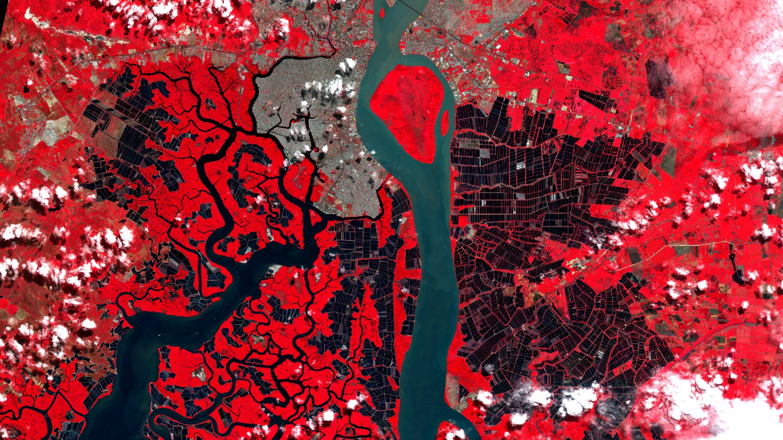
On 26 July, for the International Day for the Conservation of the Mangrove Ecosystem, the European Union space programme published a Sentinel-2 scene of the Guayas estuary in Ecuador. The caption points at the pattern that fills the landscape: “the extensive geometric features to the east and west correspond to aquaculture ponds, in an estuary where shrimp, mollusc and fish farming is performed”. And it closes with a claim about what the data can do: Sentinel-2 imagery “supports regular mapping of mangrove extent, aquaculture areas, and changes along tidal waterways”.
It names the class and does not measure it. We measured, over a box of 61.2 by 61.1 kilometers that holds Guayaquil, Santay Island and the creeks around them: 39,149 hectares of enclosed water, water that does not touch the tidal body in any of the four images. Here that is mostly aquaculture ponds, the basins where shrimp is farmed, known locally as camaroneras, but not only, and at the end we say what else fits in there. That is 10.5 percent of the box and two thirds of the 57,395 hectares taken up by the tidal body itself, river, creeks and channels included.
That number does not come from one image. It comes from four, and the rest of this piece is about how much a single one leaves out.
What the scene shows
The cover is our own recreation, built by pulling the data from the open Copernicus archive, of the same pass the European programme published, on 4 July 2026 at 15:43 UTC, with processed by T3 AISAT. It covers 52.3 by 29.4 kilometers.
It is not the same band combination as theirs. “False color” does not name one recipe, just any assignment of bands other than the one the eye uses, and the eu-space version paints vegetation green: “this false-colour image shows vegetation in shades of light and bright green”. Ours is the classic infrared combination, with the near infrared in the red channel, and in it healthy vegetation comes out red. Both are false color and both are the same data; what changes is which band goes to which channel.
The Guayas runs down the middle, turquoise from its sediment load, wrapping around Santay Island. On the left sits the pale gray fabric of Guayaquil. To the southwest lies the mangrove of the Estero Salado, deep red in this band combination, drawing a maze of meanders and tidal creeks. And on both sides, covering nearly everything that is neither city nor mangrove, the grid: huge blocks of dark rectangles separated by walls that appear as thin red lines, because they carry vegetation on top.
That grid is the subject. So are the clouds, which sit in the two right-hand corners and also along the left edge and the lower part of the frame.
The test is not shape, it is connection
Telling a pond from the creek next to it does not require recognizing rectangles. Something simpler and more robust is enough: a pond is ringed by walls, so its water does not form one continuous piece with the estuary’s.
Water is marked with the NDWI index, which compares the green band against the near infrared, and which the Space4Water portal of the United Nations Office for Outer Space Affairs reproduces from Sentinel Hub as resting on exactly those two bands: “The index uses the green and Near Infra-red bands of remote sensing images based on this phenomenon”. From all the water in the box we then take the largest continuous piece, the one you could travel end to end without leaving the water: here that is the Guayas together with the Estero Salado and its network of channels. And everything else that is water and does not touch that piece, in patches of 2 hectares or more, is enclosed water.
The test leaks in both directions, and that is worth saying before the number. A pond fills and drains through intake and discharge channels that run to the creek, so if an open channel is wider than a 20 meter pixel, that pond ends up attached to the estuary and drops out of the count: that subtracts. The other way round, anything that cuts the estuary into pieces turns stretches of river into false pond: that adds, and it gets a whole section further down because it is the big one.
What this counts are enclosures, not ponds one by one. At 20 meters per pixel a narrow wall between two neighboring ponds is not always resolved, and then the two are counted as a single piece. The 3,894 enclosures we find are therefore a minimum for the number of ponds, not the number of ponds.
How much enclosed water there is
The 39,149 hectares are spread across 3,894 enclosures with a median of 5.0 hectares, and the largest reaches 934 hectares, which is a whole block poorly separated for the reason just given. Almost half the pieces are under 5 hectares and add up to only 17 percent of the surface, while 175 large ones hold 43 percent.
| Enclosure size | Enclosures | Surface | Share of total |
|---|---|---|---|
| Under 5 ha | 1,931 | 6,682 ha | 17.1 % |
| 5 to 10 ha | 1,339 | 9,142 ha | 23.4 % |
| 10 to 25 ha | 449 | 6,620 ha | 16.9 % |
| 25 ha or more | 175 | 16,704 ha | 42.7 % |
The bottom class starts at the method’s cutoff, which on this grid falls at 50 pixels, that is 1.997 hectares and not a clean 2.000. Below that sit another 6,570 hectares of enclosed water we do not count: at that size a small pond is not distinguishable from a puddle, a ditch or an error of the index itself.
The figure also depends on where you set the index threshold and on which index you use, so we publish all four variants instead of picking one and staying quiet. Moving the threshold between -0.10 and +0.10 moves the result by 4 or 5 percent. Changing the index weighs more: MNDWI, which uses the shortwave infrared instead of the near infrared, gives 34,249 hectares, 12.5 percent less, while growing the tidal body by 12,054. Part of that gap is that it detects more water overall and part fits the intake-channel leak, and these data cannot split it. The range runs from 34,249 to 41,223 hectares: 39,149 is the value of the recipe we publish, not an exact number. And it bounds only the choice of index and threshold, not the gaps that follow.
| Variant | Enclosed water | Difference |
|---|---|---|
| NDWI with threshold 0.00 | 39,149 ha | published measure |
| NDWI with threshold -0.10 | 37,657 ha | -3.8 % |
| NDWI with threshold +0.10 | 41,223 ha | +5.3 % |
| MNDWI with threshold 0.00 | 34,249 ha | -12.5 % |
And it is worth saying what falls outside that range. The source we cite for the index warns, in the very same paragraph, about a bias that comes bundled here: “It is sensitive to built-up land and often results in over-estimated water bodies”. Guayaquil sits inside the box. We bounded it by measuring how much enclosed water falls inside a 297 square kilometer rectangle wrapped around the dense urban area: 1,866 hectares, 4.8 percent of the total. Part of that is genuine ponds pressed against the city, so 4.8 percent is a ceiling on the problem and not a correction you can subtract. That same entry puts water above 0.5 and built-up land between 0 and 0.2, and we cut at 0.00. That is not an oversight: with this estuary’s sediment load and shallow ponds, a cut at 0.5 would leave out even the river itself. Lowering it is paid for with that urban bias.
We also checked what finer detail buys. Over a test box 16.7 kilometers on a side, a single date and that date’s own geometry, measuring at 10 meters instead of 20 changes the area by 2.7 percent with NDWI and 0.4 percent with MNDWI. That says pixel size barely moves the total area; it does not say pixel size does not matter, because where the pixel really rules is the decision of whether an enclosure touches the estuary, and a single bridging pixel flips a whole piece from one class to the other. That part we have not measured.
First reason not to trust one image: cloud
Two Sentinel-2 orbits cross this estuary ten minutes apart, and only one covers it whole. Between 5 May and 29 July 2026 that orbit passed 18 times. The best of the 18 showed 69.2 percent of the box. The average across the 18 is 27 percent, and only two passes cleared half.
What we count as visible is what the product itself declares clean. Every Sentinel-2 scene ships already corrected for the atmosphere and paired with a map that labels each pixel, and which in the words of the Copernicus technical documentation holds “a classification map which includes three different classes for clouds (including cirrus) and six different classifications for shadows, cloud shadows, vegetation, not-vegetated land, water and snow”. We drop cloud, cirrus (the thin high cloud that lets light through but muddies the data), cloud shadow, snow, saturated pixels and no-data pixels, and keep the rest.
With four dates from that orbit, the four best ones, the box is seen almost in full: 91.5 percent of the surface is usable at least once, and the remaining 8.5 percent, some 31,700 hectares, we never saw clean on any of the four. That base is what carries the geometry we use, and it is why the tidal body is defined once over the union of the four passes and not date by date.
Second reason: ponds get drained
A pond emptied after harvest is bare soil, and no image counts it as water. Measuring how much that matters means comparing dates over the same surface, so we keep the part of the box visible on all four passes at once: 66,512 hectares, 17.8 percent of the total.
Inside that shared area, the enclosed water seen by the best single date is 8,469 hectares. Pooling what each of the four sees, without double counting the overlap, 9,690. The best single image misses 12.6 percent, and the worst 14.4. Only 65.9 percent of that surface held water on all four passes.
The comparison is visible to the naked eye in a block of ponds east of the river, 8.9 by 5.0 kilometers where 63 percent of the frame is pond and 96.8 percent of the pixels are usable on both dates, which leaves 2,734 comparable hectares of pond. On 19 June, 2,499 hectares held water; on 4 July, 2,423. They look almost the same, and they are not: 371 hectares changed state in those fifteen days, 223 drained and 148 filled. That is 13.6 percent of the pond surface in the frame moving between two passes.
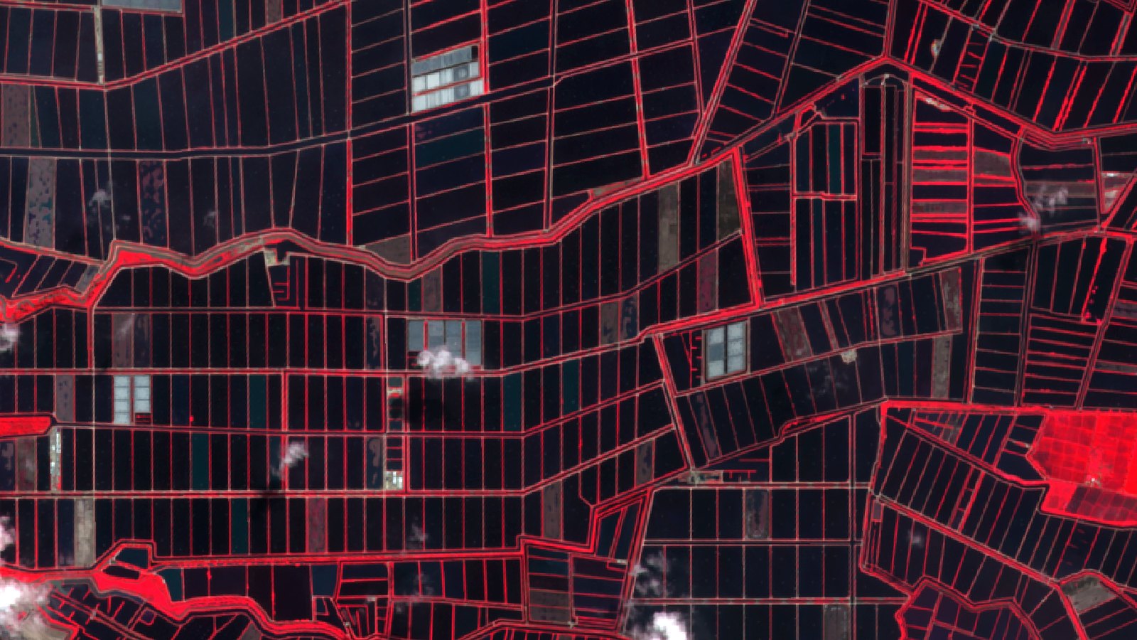
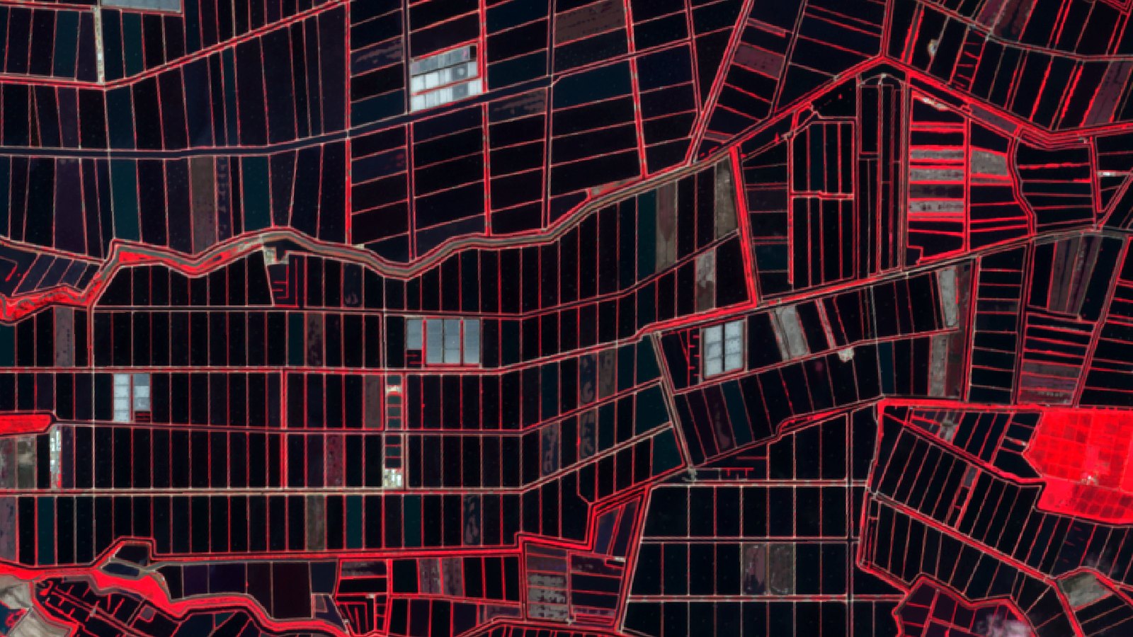
Now the part that does not flatter our own number. Of the 1,221 hectares the best date misses, only 494, or 40.5 percent, arrive as compact pieces of 2 hectares or more, the largest being 17.8. The rest comes in as narrow rims around enclosures that date already counted, and that is not a new pond: it is the same pond with a slightly lower level. Put plainly, of that 12.6 percent shortfall, about 5 points are whole enclosures that were dry and about 7.5 are edge.
The big error is not the obvious one
So far cloud takes surface away and ponds change state. There is a third effect, and it does the most damage, because it does not subtract, it multiplies.
The method leans on the tidal body being one continuous piece. A cloud lying across the river cuts it into fragments, and then the largest piece is no longer the whole estuary. The loose fragments are river, but the procedure sees water with no connection to the tide and files them as pond.
We measured it. Defining the geometry with the best scene alone, the one from 19 June, the tidal body shrinks to 24,832 hectares and enclosed water jumps to 55,170 hectares, 41 percent above the 39,149 that come out with the geometry from four dates. With one image you see less water overall and still assign far more of it to ponds. The failure is not one of precision, it is one of classification, and it gives no warning: the number comes out round, plausible and wrong.
Hence the working rule. Connectivity is defined once over the union of several passes, and only then is each date measured against that fixed geometry. It is the same discipline we applied when comparing two scenes of a tidal coast: what changes between images has to be the phenomenon, never the surface you evaluate.
What this measurement does not say
It does not say how much mangrove there is. Separating mangrove from other riverside vegetation with a single optical scene is not reliable, and we did not try: the cover scene shows the mangrove of the Estero Salado, but showing is not measuring.
It does not say that all of that water is shrimp. It also takes in closed lagoons, irrigation reservoirs, salt pans and freshly flooded rice. All these data let us rule out is water with a canopy on it: the vegetation index inside the enclosed water averages between -0.11 and -0.26 depending on the date, on a scale from -1 to +1 where living vegetation climbs past 0.2, and under 2.1 percent of those pixels get there. It is open water. A rice paddy just flooded is open water too, and that one is not separated without crossing against a land use map or the full year of the series. It is the first pending improvement.
Nor does it say how many ponds there are, because of the unresolved wall. That needs finer detail or a radar sensor, and it is a different measurement.
The 39,149 hectares are also everything that showed water on at least one of the four dates in June and July, not a state: a pond dry on all four passes is invisible here, and the index pushes the same way, because over very turbid water it drops and can fall below the threshold.
And there is the tide. The 57,395 hectares of channel are the accumulated geometry of the four passes, not an instantaneous water surface; the pond figure is far less sensitive, precisely because a wall isolates it from the tide.
What decision this supports
Anyone watching aquaculture surface wants to know how much is there, and also how much is in production. The first is answered with a stable geometry from several passes; the second, with the time series on top. Measuring with whichever month came out clearest answers both with the worst available tool.
There is money on the table. Ecuador’s national aquaculture body put 2025 shrimp exports at USD 7.47 billion, 23.2 percent above 2024, and in that same report an industry figure describes it as the world’s largest exporter. Around that figure sit concessions to inspect, certifications to audit and no-expansion commitments over mangrove that somebody has to check. A 13 percent difference in the surface you count, or 41 percent if you also get connectivity wrong, is not a methodological footnote: it is the difference between a file that holds up and one that does not.
The procedure that follows from this is short. Define the connected water body over the union of at least four clean passes. Measure each date against that fixed geometry. And publish the split by how many observations held water, because telling an active pond from a resting one is worth as much as the total.
What we build with this
Mapping ponds from orbit is a known exercise, and recreating a scene and computing an index is the easy part. What we put together at T3 AISAT for fisheries and aquaculture, water and farming is the whole step: choosing the passes that work, fixing the geometry, measuring the series, publishing the sensitivity and writing down the procedure so that six months from now it returns a comparable number and not a new one. The same discipline with which we measured what the European wildfire statistics leave out, applied here to an estuary.
If you had to declare the aquaculture surface of your area next month, how many images would you count it with?