By Pedro Hernández
A hillside olive grove has two surface areas, and both are true. One is the area the map draws: the shadow of the ground on a flat plane, as if it were level. The other is the area walked by whoever works it, and on a slope it is always larger. The EU’s Common Agricultural Policy, the CAP, and the cadastre measure the first one. The tractor, the dose per hectare and the yield all work on the second.
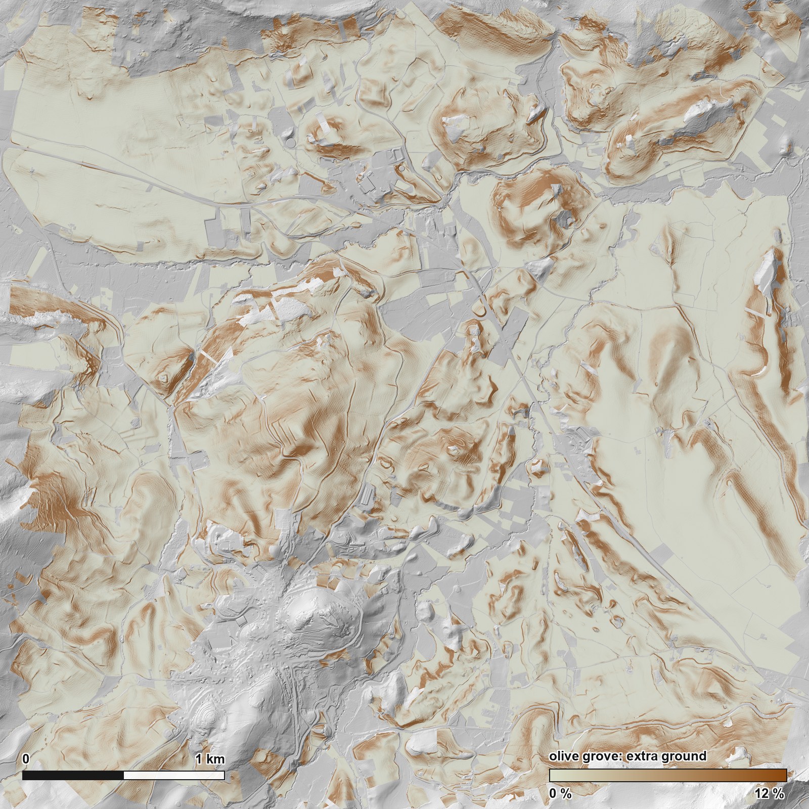
In the Sierra Subbetica of Cordoba, Spain, SIGPAC, the official map behind CAP aid, publishes 1,363.84 hectares, and the 2024 public airborne laser scan finds 1,408.32 hectares of real ground there, using squares 2 meters on a side: 3.26 percent more. That is 44.5 hectares of difference over the 1,364 measured. Where the slope passes 50 percent, that gap rises to 18.5 percent on average.
Of those 1,364 hectares, 1,051 are olive grove, a little over three quarters; the rest is mostly fruit trees, pasture and unproductive ground, and then the town itself, arable land and tracks. The 3.26 percent covers the whole measured set. If you take away one number and yours is olive grove, take the olive grove one: 2.83 percent. It comes out lower because the olive grove in this frame is a little less steep than the average.
Two words worth keeping apart from the start. The frame is the measured window, 4 kilometers on a side, with Carcabuey in its southwest quadrant and Priego de Cordoba about 6 kilometers to the east. The parcels are what sits inside it: a parcel here is the unit SIGPAC uses to split a holding by land use, and SIGPAC is the official map of Spanish farm parcels, on which CAP aid is processed. The airborne laser scan, or LiDAR, flew in 2024 and swept the ground with light pulses. Over this area it left 9.7 measured points per square meter, nearly twice the minimum of five the product declares. Those points build the terrain model, a grid of squares each carrying one height. Here those squares, the cells, are 2 meters on a side.
Neither surface area is wrong
They answer different questions. The projected area says how much map a holding takes up: it is what hands out aid and what the cadastre holds. The real area says how much ground there is to plow, treat and harvest, and planting density, dose per hectare and yield all hang off it. On flat ground the two match. On a slope they do not.
The 3.26 percent is spread very unevenly
The average hides the result. Sorting the 2,563 measured parcels by their slope, the extra ground runs from almost nothing to almost a fifth:
| Mean slope of the parcel | Parcels | Extra ground | Map hectares |
|---|---|---|---|
| 0 to 5 % | 206 | 0.14 % | 84.9 |
| 5 to 10 % | 454 | 0.52 % | 234.1 |
| 10 to 20 % | 730 | 1.66 % | 422.5 |
| 20 to 30 % | 594 | 3.84 % | 358.9 |
| 30 to 40 % | 371 | 6.72 % | 193.3 |
| 40 to 50 % | 125 | 10.28 % | 50.0 |
| over 50 % | 83 | 18.53 % | 20.2 |
The parcels add up to 2,563 and the hectares add up to the 1,364 measured, so the table is complete. One warning about the percentage column: each row is the average of the parcels in that band, counting a half hectare parcel the same as a twenty hectare one, while the overall 3.26 percent is weighted by hectares. That is why averaging the seven rows by eye does not return the total.
The shape of the table is predicted by geometry, with nothing measured. A 30 percent inclined plane has 4.4 percent more ground than its flat base: it is the long side of a triangle with a base of 100 and a height of 30, which measures 104.4. Our parcels sit consistently above that curve, and the correlation between measured and theoretical is 0.989. What is left over is the relief each parcel has inside it, which its mean slope does not capture. It is the same ground to map ratio that Jenness showed how to compute from terrain models in 2004 for habitat studies.
The next figure keeps only the olive grove: 1,743 of the 2,563 parcels, of which it plots 1,738, because five fall outside the axes.
One caveat about scope. The 3.26 percent is the excess of the parcels that fit whole inside the frame and reach 1,000 square meters. The ones cut by the edge are dropped, because the area SIGPAC publishes for them refers to the whole parcel. That leaves out steeper ground: the 413 parcels the edge cuts have a 26.2 percent mean slope, weighted by hectares, against 20.0 percent for the ones that stay inside. That is part of why the whole frame gives 3.49 percent and the measured parcels give 3.26 percent: the frame also holds ground that belongs to no parcel, and the smallest parcels.
Averaging the slope first loses almost nine hectares
There is a fast way to do this sum. It gets used a lot, and it always falls short. It takes the mean slope of the parcel, applies the matching correction and multiplies. The trouble is that the correction grows faster than the slope.
Picture a holding that is half flat and half on a 60 percent slope. Its mean slope lands on a middle value that exists nowhere on the holding, and the steep part adds far more ground than that average lets on.
Measured here: adding up cell by cell gives 1,408.32 hectares, and that shortcut gives 1,399.35. The difference is almost nine hectares, 0.64 percent of the real area. These are not hectares missing from our count: they are the ones anyone taking the short route would leave behind. And they would leave them behind in all 2,563 parcels, without a single exception possible, because that correction grows faster than the slope.
Real surface area is not one number: it is one number per ruler
A rough surface has no single area. It has one area per cell size used to measure it, just as a coastline has no single length: the shorter the ruler, the more inlets it picks up and the longer it comes out.
Redone at different cell sizes, the excess runs from 4.34 percent with half meter cells to 1.80 percent with 50 meter cells. These figures cover the whole frame and not the measured parcels, which is why they do not match the 3.26 percent from the start.
That calls for a control: running the same calculation somewhere you already know what should come out. Here that somewhere is the almost horizontal ground, and it is the lower curve in the figure. Geometry predicts an excess of 0.011 percent there, practically zero. But what half meter cells actually measure is 1.17 percent: a hundred times what geometry predicts.
That gap has a tempting and wrong name, which is to call it model error. Looking at what is actually in those flat cells turns up walls, banks and ditches: real ground. So the 1.17 percent is a ceiling, the worst that could be left over, and not a measurement of what is left over.
That ceiling comes down once the calculation is matched to what we do here: first by cell size, from half a meter to 2 meters, and then by ground type, keeping only flat olive grove, which is the comparable case. These are the four figures for the frame at a 2 meter cell size, and they are worth keeping apart:
| Excess measured with 2 meter cells | |
|---|---|
| The whole frame | 3.49 % |
| Only the measured parcels, which is this article’s figure | 3.26 % |
| Control: only where the ground is flat | 0.56 % |
| Control: only flat olive grove | 0.29 % |
0.29 percent is the ceiling the olive grove gets, and it is still a ceiling: it is not subtracted. Even if someone took it whole off the 2.83 percent, what is left stays above 2.5 percent.
So we work at 2 meters, and that has to be said out loud: it is a choice, and it is declared. At that size the control has already halved. Publishing the 4.34 percent from half a meter without this figure would mean calling hillside relief what at that size is mostly wall, ditch and the grain of the model itself.
What the SIGPAC contrast checks, and what it does not
The check that counts is the slope one. SIGPAC publishes a mean slope per parcel, computed by a different agency and with a different procedure. Spanish Royal Decree 1047/2022, in letter i of its article 2, defines it as computed from the reference digital elevation model of the national geographic institute, using neighboring cell analysis. Set against ours over the 2,563 measured parcels, the correlation is 0.9879. It is a different comparison from the one above, even though the number looks alike: that one set our measured ground against what geometry predicts, and this one sets our slope against the slope another administration publishes. We could not find out which flights that official model comes from, so we do not know whether the two measurements share raw material. If they did, the agreement would prove less than it seems: two measurements that start from the same data can be wrong in the same way.
Ours comes out half a point larger at the median, and the scale curve explains the direction: the finer you measure, the more relief shows up. What we cannot claim is which of the two is closer to the ground, because that decree fixes the model and the method but not the cell size.
And a correlation without saying what it was computed on is half a truth. The 0.9879 is over parcels of at least 1,000 square meters. Over the 4,830 whole parcels in the frame, which are those same ones plus the parcels below that size, it drops to 0.9511: across a few square meters a mean slope is poorly defined.
The second check looks like it validates our measurement of the ground, and it does not. It measures the outline SIGPAC draws and compares it with the area SIGPAC itself declares for that outline. The median error is 0.000000 percent, and that zero is expected: the same number is computed twice from the same source. It does not validate our measurement of the ground. It is a reference control, and that is the name it gets.
What it does prove is two things. That we work in the same coordinate system and the same units. And that the map measures the shadow of the parcel on a flat plane, on purpose: here the flat map shrinks what it draws, so measuring that same outline on the curved Earth would give 0.67 hectares more over the 1,364, which is 0.05 percent, instead of zero. The three rows in the figure are three ways of measuring the same thing, not three amounts that add up.
Parcel slope is a condition for aid
This is where it stops being a geometric curiosity: the mean slope of the parcel and the trees per hectare are conditions for receiving aid. And the hectare that counts in the file is the one SIGPAC publishes for the parcel, which is the area of its outline on the map, as the control above has just checked. Spanish Royal Decree 1048/2022 reserves, in its version now in force, the coupled aid for olive groves with specific difficulties and high environmental value to parcels classed as rainfed land in SIGPAC. On those parcels it requires, in its article 79 and among other conditions, a planting density of up to 100 trees per hectare, or a mean parcel slope of 25 percent or more. The two conditions sit in the same sentence and are joined by an or, so meeting either one is enough. The slope branch is the one developed here, because it is the one measured with the terrain model. The density branch is measured by counting trees, and the next article in this series counts 124.3 olive trees per hectare from the same flight.
Note which way that condition runs, because it reads backwards from what you expect: the aid is for thin or steep groves, so that condition is met at 100 trees or fewer, or at 25 percent slope or more. Put the slope threshold on our own data and the border is crowded. There are 96 olive parcels with a mean slope between 24 and 26 percent, on either side of the line, inside a band as wide as the typical gap between two ways of measuring slope. That count does not separate rainfed from irrigated ground, which is the first thing the case file looks at.
And it is worth saying which way our bias pushes, before someone else says it. Our slope comes out half a point above the official one, so a parcel of ours looks steeper than SIGPAC says it is. With our numbers the 25 percent threshold is easier to meet. None of this makes our measurement the right one. It says that at that threshold the choice of model and of cell size stops being a method discussion and starts moving case files.
How far this goes
This does not replace a surveyor. A boundary settlement, a registry entry or a boundary dispute needs a field survey signed by a qualified professional, with instruments that fix centimeter coordinates on the ground itself. What is measured here is the size of the effect across sixteen square kilometers. It certifies no holding and it does not say where a boundary line runs.
The terrain model is provisional, and its own publisher says so. Spain’s National Center for Geographic Information warns that these half meter models come from an initial classification of the point cloud and that a final version is planned, built from more advanced classifications, which the center says will improve the quality and reliability of the final product. When it arrives these surface figures will have to be redone.
One effect pulls the other way and we do not know which wins. Of the 9.7 points per square meter the flight leaves, only some land on the ground, and under the crowns far fewer: on one of the one kilometer squares that the data comes in, 3.10 ground points per square meter under crown against 5.22 outside. The ground under the olive grove is reconstructed from less information and comes out smoother, so the fine relief is somewhat underestimated exactly where the olive grove is measured.
And none of this says whether the olive grove is healthy or whether it produces. Vigor, this season’s crop and abandonment were not measured. The ground was measured.
Two columns, not one
The area that collects the aid is already yours, by province, from the SIGPAC download service. The one that governs dose, density and yield is the real area, and in this olive grove it runs 2.83 percent above the other, with four single parcels past 20 percent. Put on a single holding: in the 30 to 40 percent slope band, where the average excess is 6.72 percent, an olive grove of 10 map hectares has almost 7,000 square meters more ground to work. That is the kind of data we put into a parcel by parcel monitoring panel: the area that collects and the area that gets worked, each in its own column, so that nobody mixes them up.
The input data is public and the arithmetic is ours. Anyone who redoes it in their own area with a different cell size will get a different number, and that is exactly the interesting part.
It is the same mix-up as on the Rhine, where the satellite measures the width of a river and not its navigable depth, which is the depth that decides how much cargo a barge can carry. Two quantities that look alike and do not substitute for each other. What is missing here is the other half of the frame, the trees. The same laser scan that measured the ground also leaves the height of every crown, and the next article in this series counts 130,668 crowns with it in these same parcels.
There is one question no image answers: when your organisation works out a dose per hectare, a yield or a planting density, do you know which of the two surface areas sits under that number?
Data: terrain model and point cloud, the loose heights the laser returns before they become a grid, from the LiDAR flight of the Spanish national aerial imagery program, obra derivada de MDT50cm-cob3 2022-2025 CC-BY 4.0 scne.es and obra derivada de LiDAR-PNOA-cob3 2022-2025 CC-BY 4.0 scne.es; Recintos SIGPAC campaña 2026 © FEGA (CC BY 4.0). The acknowledgement wording is fixed by the Spanish licenses and is left in Spanish on purpose.
How this was made. Everything measured here comes from official public data, the sources above, each with its licence. Every figure was checked against those sources before publication.