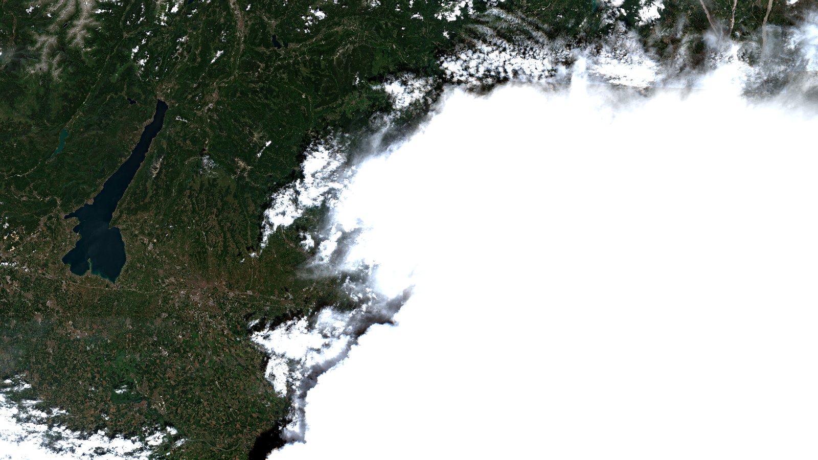
On 22 July, the Copernicus image of the day published a convective storm over northern Italy. The caption explains the V shape of the cloud top like this: “It forms when powerful rising air carries the storm cloud to high altitudes, at which strong winds split and flow around the cloud top”. High. That word does all the work in the sentence, and it carries no number.
The number is in the picture itself: a cloud that tall casts a long shadow, and a shadow is a ruler lying on the ground. We rebuilt the scene from the Copernicus Data Space Ecosystem and measured it. The answer is not a number, it is a table. The height depends on where you decide the cloud ends: about 8 kilometers if you count the whole sheet, and 12 to 14 if you keep only the dense core, the candidate for the anvil top. That dependence is what a single optical frame can give, and explaining it is half this article.
Our scene, and the time that is not the time
The lead image is that same pass, rebuilt by us over a frame of about 218 by 123 kilometers, with Lake Garda on the left, the Po plain below and the Prealps above. True color (B04, B03 and B02) and processed by T3 AISAT, with a hard tone curve: there is a factor of ten in reflectance between a sunlit anvil and a shaded plain, and both have to be readable in the same image.
The first surprise shows up before you look at a single pixel. The original caption says the image was taken “on 21 July 2026 at 10:05 UTC”. But that time is not a measurement: it is the one in the file name, which marks the start of the pass. Ask the Copernicus catalog which tiles cover the Veneto that day and you get twelve, from two satellites. The nine Sentinel-2B tiles carry their real observation time, and none of them matches the caption: they run from 10:17:53 to 10:18:28 UTC.
That 10:05:59 in the file name is not the time of the picture. The Sentinel-2 product documentation on SentiWiki says so plainly: “The first date (YYYYMMDDHHMMSS) is the datatake start sensing time”. A datatake is “the continuous acquisition of Sentinel-2 image data in a given MSI mode” and it can run up to 15,000 kilometers, so the moment it starts falls very far, in time and in space, from the piece of the world you care about. Here, twelve minutes.
Twelve minutes is a detail if you are looking at a corn field. Over a storm that, by the original’s own account, “developed in the early hours of 21 July”, it is a different storm, and if you plan to match the image against radar or a damage report, that offset goes straight into your conclusion. The catalog shows something else: two Sentinel-2 satellites flew over that morning ten minutes apart, but the 2A swath, at 10:28 on relative orbit 065, stays west and never reaches the storm. It is the same mismatch between file name and real observation time that we documented over the Guinea-Bissau estuary, where twelve minutes decide which tide phase you are looking at.
A shadow is a ruler
The idea is basic geometry: if you know how high the Sun is and a cloud casts a shadow of length L, the height of the cloud comes out of a triangle. What makes this work with Sentinel-2, rather than with any photo, is that the product ships the geometry already measured. Every L2A scene includes the solar and viewing angle grids, so you do not compute the position of the Sun, you read it.
Over our frame the product declares a solar zenith of 26.76 to 29.33 degrees, that is a Sun between 60.7 and 63.2 above the horizon, and a solar azimuth of 145.4 to 152.4. With the Sun in the southeast, the shadow falls to the northwest.
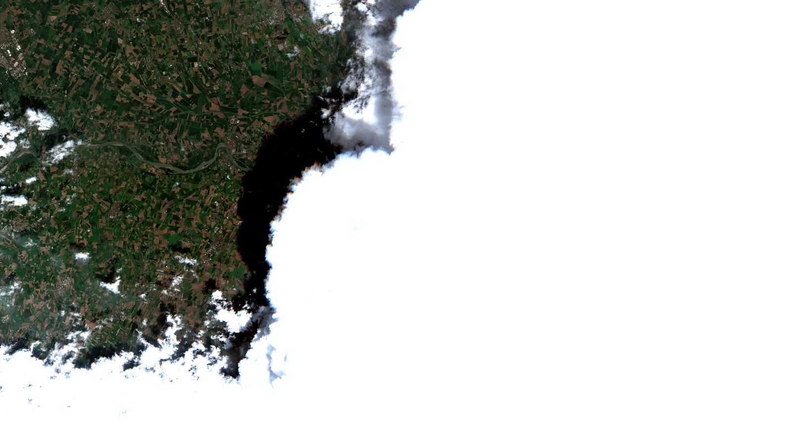
That black band is the ruler.
First the direction, and without assuming it
Measuring the width of that band by eye would give you a number, and just as easily a wrong one: the edge of the cloud is not straight, the shadow falls at an angle, and the eye picks the spot that suits it. So we did it over the whole scene, in two steps.
We downloaded the frame as reflectance, with no gain and no curve, at 120 meters per pixel. Anvil is anything above 0.80 of brightness in the blue band, 38.6% of the scene; clear ground is anything below 0.18, 35.7%. The threshold looks odd because surface reflectance goes above 1 over a cloud: the atmospheric correction is built for ground, so up there the value only works as a brightness measure. Then, for every azimuth from 0 to 350 degrees, we take the strip of ground within 2 kilometers of the cloud in that direction and average its brightness. Brightness here, and throughout the article, is the mean of the three bands we downloaded: blue, red and near infrared, not just the blue used for the masks.
If what we are seeing is a shadow, there has to be a single dark lobe, and its axis has to fall where the Sun says. That is what comes out:
| Direction from the cloud | Mean ground brightness within 2 km |
|---|---|
| 150 degrees (toward the Sun) | 0.1668 |
| 110 degrees | 0.1658 |
| 200 degrees | 0.1641 |
| 290 degrees | 0.1358 |
| 320 degrees | 0.1256 |
| 330 degrees | 0.1254 |
| 340 degrees | 0.1274 |
| 350 degrees | 0.1307 |
| 10 degrees | 0.1375 |
| All clear ground in the scene | 0.1512 |
(Extract. The full sweep covers 36 directions, one every 10 degrees.)
One minimum, and it sits where it should. The vertex of the parabola through the three lowest points falls at 326.0 degrees; the anti-solar azimuth the product declares is 328.7, and the full model below, with parallax, predicts 323.4. Our measurement lands between the two, less than three degrees from each, and cannot tell which is better: the floor of the lobe is too flat. What it does establish is that the Sun sets the direction of the darkening.
Look at the other end of the table: toward the Sun, the ground next to the cloud comes out brighter than the scene average. That is the null test. If the strip beside the cloud came out dark in every direction, we would be measuring an artifact of our sampling, not a shadow.
Then the length
The second step is the profile: mean ground brightness in half-kilometer bins, minus the same profile along the two perpendiculars, which act as controls. The shadow lasts while that difference is negative and ends where it returns to zero.
| Distance from the cloud | Ground along the shadow | Mean of the two controls | Difference |
|---|---|---|---|
| 0.25 km | 0.1270 | 0.1661 | -0.0390 |
| 0.75 km | 0.1211 | 0.1560 | -0.0348 |
| 1.75 km | 0.1312 | 0.1527 | -0.0215 |
| 2.75 km | 0.1391 | 0.1515 | -0.0123 |
| 4.25 km | 0.1419 | 0.1505 | -0.0085 |
| 5.25 km | 0.1460 | 0.1497 | -0.0037 |
| 6.25 km | 0.1526 | 0.1525 | +0.0002 |
| 7.25 km | 0.1588 | 0.1517 | +0.0071 |
(Extract. The full profile has 26 bins.)
The zero crossing lands at 6.23 kilometers. Along the anti-solar direction the product declares it gives 6.37: those not quite three degrees move the result by 2%.
The satellite’s own parallax
This is where the easy sum falls short. A cloud top twelve kilometers up is not drawn above its own vertical. The product is orthorectified for the terrain, so the line of sight from the satellite to the top carries on until it meets the ground, and that meeting point sits offset away from the satellite. That is a triangle, not a Copernicus quirk. And that a high object is not placed correctly in a Sentinel-2 product is something the house does say. SentiWiki warns, in its section on instrument parallax effects, that “the processing algorithm ensures the co-registration of images acquired by all spectral bands and the detectors for features at ground level. Objects at a higher altitude like planes and clouds cannot be properly co-registered”.
The viewing zenith runs here from 1.05 to 11.79 degrees, with a mean of 4.12 over the anvil pixels, and that mean is the value we apply. At that angle a twelve kilometer top shifts by 0.9 kilometers; at the edge of the swath it would shift by 2.5. So the distance between the cloud and its shadow is the sum of two displacements, and the height comes from dividing the measured length by the magnitude of that sum.
With the Sun alone, 6.23 kilometers of shadow and a solar zenith of 27.76 degrees over the anvil give 11.8 kilometers; with the parallax term, 10.8. The second is more complete but more fragile: the satellite switches sides across the swath, so a viewing azimuth averaged over the whole scene describes no pixel well. We publish both and keep the interval.
The number, and what it is not
Everything above rests on a decision of ours: calling cloud anything above 0.80. Let us change it. Nine threshold combinations, with the height computed case by case:
| Cloud threshold (B02) | Ground threshold (B02) | Shadow L (km) | h with parallax (km) | h from the Sun alone (km) |
|---|---|---|---|---|
| 0.60 | 0.14 | 4.89 | 8.42 | 9.29 |
| 0.60 | 0.18 | 5.04 | 8.68 | 9.57 |
| 0.60 | 0.22 | 5.13 | 8.82 | 9.73 |
| 0.80 | 0.14 | 6.09 | 10.55 | 11.56 |
| 0.80 | 0.18 | 6.23 | 10.79 | 11.83 |
| 0.80 | 0.22 | 6.32 | 10.95 | 12.00 |
| 1.00 | 0.14 | 7.16 | 12.45 | 13.63 |
| 1.00 | 0.18 | 7.26 | 12.62 | 13.82 |
| 1.00 | 0.22 | 7.52 | 13.07 | 14.31 |
The ground threshold barely matters: it moves the height by less than half a kilometer. The cloud threshold changes everything, and in an orderly way: the stricter it is, the taller the cloud comes out. Not noise, but the method telling the truth about itself, because the shadow is cast by the edge of whatever you called cloud and that edge is not always at the same height. At 0.60 the outline lands on the thin sheet around the storm; at 1.00, inside the dense core, the part that actually went up.
So the result is not one number. It is two:
- The optical core of the storm, the candidate for the anvil top, casts a shadow that puts it between 12 and 14 kilometers.
- The sheet around it, counting all the bright cloud, comes out between 8 and 12.
Both are for 10:18 UTC on 21 July 2026, over the west flank of the complex, and this scene will not narrow the bracket: that would take another instrument.
Three warnings, because the numbers are worth less without them:
- Each figure is the height of the outline we chose, averaged over a complex more than a hundred kilometers across. Not a local peak, and not the maximum top, which may sit higher.
- Deep in the shadow, L2A reflectance bottoms out: of 3,208,776 valid pixels, 9,400 have B02 exactly 0, which is 0.29%, and 1,393 have it in all three downloaded bands, 0.04%. Too little to move the profile, but the radiometry inside the shadow is gone. SentiWiki also documents that “due to inaccuracies of the Digital Elevation Model, a strong terrain correction may be applied in totally or partially shaded areas”, with “inaccuracy in the surface reflectance” as the result.
- It is not a radiosonde and not a radar echo, but an optical measurement from a single pass, with its method declared and its bracket published.
What it supports, and what it does not
The first decision is a negative one: Sentinel-2 is not the tool for watching a storm. Geostationary sensors are built for that, and EUMETSAT says as much about the imaging services of its third generation Meteosat: “Nowcasting applications are the focus of the imaging services”, with lightning detection delivered in 120 seconds. A low orbit satellite gives you one picture and leaves.
What it does add is geometry at ten meters and a measurable height, and that connects to risk. The overshooting cloud top detection page of the EUMETSAT convection group sums up why the top matters. It is written by Kristopher Bedka, of NASA Langley Research Center: “Storms with overshooting tops (OT) typically generate hazardous weather conditions such as hail, damaging wind, tornadoes, and flooding”. Those tops show up near “~60% of wind, hail, and tornadic storms”. The original already warned that the V pattern goes with storms able to produce “destructive wind gusts, large hail, and torrential rainfall”, and that this one hit Vicenza, Padua, Rovigo and Treviso. It is the same emergency logic behind how we measured wildfire severity with the NBR index in Cinco Villas: the image alone is not enough, you need the number and its method.
So the order is this: the geostationary sensor tells you when and where it is happening, the high resolution optical sensor tells you on the next pass where the mark was left, and the geometry of the storm day scene helps bound the severity. Mixing them without checking the clock is the easy way to pair an image with the wrong radar trace.
What we build with this
At T3 AISAT we build, for the emergencies sector, observation chains that run all the way to a decision: catalog, reproducible scene, measured index and the alert that goes with it. This article sums up the dull part of the job: read the angles the product already ships, check the tile time instead of the file name, and publish the null test next to the result. Nothing here needs private data: it all comes from the open Copernicus archive, which is why anyone can redo it.
How many of the satellite images you work with carry a time nobody has checked?