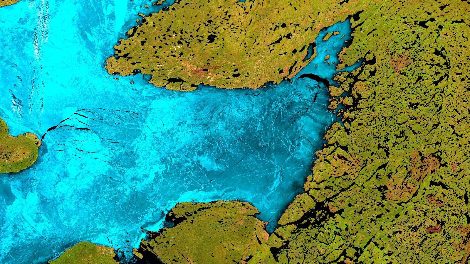
On 10 July 2026, ESA published Great Bear Lake in its Earth from Space series, using a Sentinel-2 scene from 17 June. The text walks through five colors and what each one means: ice in blue and cyan, water in dark blue or black, land in greens, orange and pink patches of bare rock, and black cracks across the ice sheet.
It explains the image like this: “In this false-colour image, three specific bands from Copernicus Sentinel-2’s visible and infrared channels have been used to process the image.”
Three specific bands. Which ones, it never says. We read the whole page: there is no band identifier anywhere, no B4, no B8, no B11. Without the recipe you cannot rebuild the image, you cannot check any of the five color readings, and you cannot run the same method over another lake next week.
So we rebuilt it.
What our scene shows
We recomposed the frame from the Copernicus Data Space Ecosystem, using the same day ESA declares: 17-06-2026. The frame is 241 km east to west by 136 north to south, at about 151 meters per pixel. It crosses several satellite passes, so the image is a mosaic of that day’s takes, not a single one. And it covers the center and east of the lake, not the whole lake: ESA gives the full area, 31,328 sq km, “the largest freshwater lake entirely within Canadian borders”, with ice “from late November through to July”.
The framing was settled by eye, not by a filter. Our first attempt reached about 150 km further west and came out with two defects: a black wedge with no data, which is the edge of the satellite pass, and a bright, textured band over the western shore. No number caught either one; both are obvious the moment you open the file. Over the frame we did publish, the catalog returned twelve takes for that day and all twelve declare 0.0% cloud, so here the cloud filter had nothing to remove.
The central ice reaches the shore in the north and pulls away in the east, opening a continuous band of clear water. ESA names it well: “creating a clear moat of ice-free water between the land and the remaining ice sheet.” And black fractures cut across the sheet from side to side.
Three bands, and a testable guess
ESA’s page leaves a clue. Explaining the color of the ice, it writes: “This range of colours is due to ice and snow having a higher reflectance in the visible part of the spectrum, here assigned to blue.” So the blue channel of their composite carries a visible band.
It is worth saying here what ESA takes for granted, because it is the whole trick. A screen has only three channels: red, green and blue. Sentinel-2 measures in thirteen bands. Building an image means choosing which band feeds which channel, and nothing more. The color you see is not the color of the scene, it is the result of that assignment. True color picks the three bands that match our eyes. False color picks something else, which is exactly why you need to know what. It is the same idea we explored with the Egyptian irrigation pivots that near infrared paints red.
That clue alone does not rule out the color infrared composite, the one that paints vegetation red, because it also carries a visible band in blue: it is red equals B08, green equals B04, blue equals B03, and B03 is the green band. What rules it out is the result. With that recipe the surrounding land would come out red, and ESA describes the opposite, “shades of green dominate the landmass surrounding the lake”. And the ice, with the reflectances we measure below, would land at 0.306 red, 0.364 green and 0.381 blue: a near neutral gray, not the blue and cyan of their text.
There is another classic combination that fits both the clue and the use their page states, “monitoring ice melt, water bodies and vegetation health”: red equals B11, green equals B08, blue equals B04. According to SentiWiki, the official Copernicus documentation, B04 is visible red at 665 nm and 10 meters, B08 is near infrared at 842 nm and 10 meters, and B11 is shortwave infrared at 1610 nm and 20 meters. The same page states what the two SWIR bands are for: “2 wider SWIR bands (~1610nm and ~2190nm) for applications such as snow/ice/cloud detection, or vegetation moisture stress assessment”.
This is a guess, not an attribution. We do not know what ESA used and we are not going to claim we do. It is not the only candidate either: B12, B11 and B04 also leaves a visible band in blue and would also turn the ice blue, because B12 behaves like B11 over snow. What you can do with a guess is generate it over your own scene and see whether it reproduces, one by one, the five color behaviors ESA’s text describes.
The reflectances, measured
Looking at the image and saying “yes, that matches” checks nothing. So we downloaded the same scene as reflectance, with no gain and no enhancement curve, on an 800 by 450 grid. Reflectance is the fraction of incoming light a surface sends back, on a scale of 0 to 1, and here it is surface reflectance, already corrected for the atmosphere, which is what the L2A label in the image caption means. With that we sorted all 360,000 pixels using four threshold rules. They run in cascade, each pixel falls into the first rule it meets, and we publish them so anyone can redo the count: water if B08 and B11 both fall below 0.05; ice if B04 is above 0.25 and B11 below 0.15; vegetation if B08 is above 0.18 and more than 1.8 times B04; bare rock if B11 is above 0.16 and B08 below 1.8 times B04.
| Class | B02 blue | B03 green | B04 red | B08 NIR | B11 SWIR | % of scene |
|---|---|---|---|---|---|---|
| Ice and snow | 0.3957 | 0.3807 | 0.3636 | 0.3063 | 0.0134 | 32.6 |
| Vegetation | 0.0390 | 0.0567 | 0.0521 | 0.2103 | 0.2076 | 31.0 |
| Open water | 0.0164 | 0.0172 | 0.0118 | 0.0068 | 0.0064 | 7.2 |
| Bare soil and rock | 0.1280 | 0.1352 | 0.1328 | 0.1357 | 0.2358 | 1.5 |
| Unclassified | 0.1209 | 0.1234 | 0.1153 | 0.1543 | 0.0889 | 27.7 |
That 27.7% unclassified belongs in the table because it is part of the result. The measurement grid is 800 by 450 over the same 241 km, which works out to about 301 meters per pixel: the shoreline, melting ice and wet ice fall between thresholds, and a crude threshold leaves out whatever sits on the edge. At 300 meters per pixel there is more mixing, not less.
Each color against its number
Now ESA’s five readings can be checked with numbers instead of impressions.
Ice in blue and cyan. Ice reflects 0.3636 in visible red and 0.0134 in SWIR: twenty-seven times less. Since B11 goes to the red channel and B04 to the blue one, red goes dark and blue lights up. Near infrared fills the middle at 0.3063, and that is where the cyan comes from. This is exactly the snow signature the National Snow and Ice Data Center describes, “very high visible (VIS) reflectance and very low reflectance in the shortwave infrared (SWIR)”, and the basis of the NDSI snow index.
Vegetation in green. Near infrared rises to 0.2103 while red stays at 0.0521, four times lower. B08 drives the green channel and the result is olive green, with one twist: vegetation is also high in SWIR, 0.2076, so the red channel contributes and the green leans yellow. You can see it in the image.
The orange patches. This is the only class where SWIR is the highest of the five bands, 0.2358. Red channel dominant, and out come the rust orange patches. It pays to quote ESA in full here, because they do not pin these on one thing: “indicating exposed rocky terrain, typical of the Canadian Shield, sparsely vegetated tundra or older fire scars that have not yet fully revegetated”. Bare rock, thin tundra and old burn scars share a spectral signature, and these five bands do not tell them apart.
Water in black. All five bands stay below 0.02, the lowest of any class. Three channels dark at once: black. ESA explains it the same way, “because water reflects very little light back to the satellite, it appears dark blue or black”.
Four out of four. ESA’s fifth reading, the cracks, is the water case again: a fracture is open water, so it comes out black against the ice.
What true color hides
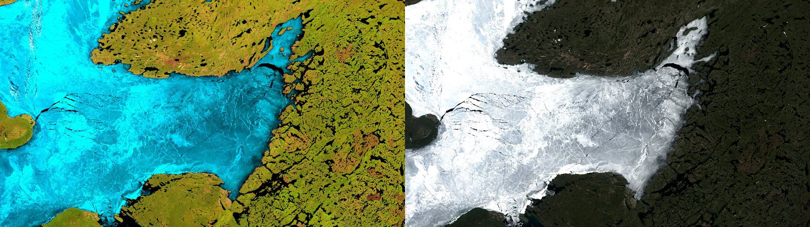
In true color, the ice on Great Bear Lake is white. And it is not white by accident: its three visible bands measure 0.3957, 0.3807 and 0.3636, almost the same value. Under 9% between blue and red is all the color there is. That is why the whole sheet comes out as one bright, flat mass, and why the surrounding land, which reflects seven times less in the red and ten times less in the blue, sinks into a green so dark it reads as black. The tone curve that keeps the ice from burning out crushes the forest.
There is a fair objection here: of course, you gave true color the same curve as the false color version. True, and on purpose, because if each version gets its own adjustment the comparison stops measuring the bands. With its own curve the forest would lift, certainly. What no tone adjustment can do is change the order of the surfaces, and that order is the argument.
Because what SWIR adds is not magnitude, it is order. It does separate: 15.5 times between ice and vegetation at B11, against 10.1 in visible blue. But blue separates in the same direction as the rest of the visible, and B11 separates in the opposite one. Across the first four bands ice sits above and vegetation below; at B11 ice drops to 0.0134 and vegetation holds at 0.2076, fifteen times higher. A channel that flips the order adds color, not just brightness, and that is why a composite carrying SWIR separates surfaces that true color runs together.
Two things we will not claim
ESA says the ice tones run “from bright blue to cyan, depending on the ice thickness”. Our scene is a single day and it does not separate thickness from snow cover, surface melt or roughness. The tone does vary, clearly. Pinning that variation on thickness with one image is a different claim, and we are not making it.
One more note on their text. The same page calls Great Bear Lake “the largest freshwater lake entirely within Canadian borders” and, a few lines later, describes “a massive sheet of sea ice covering most of the lake”. This is lake ice. The distinction matters because lake ice and sea ice neither form nor break up the same way: lake ice is not driven by ocean currents or salt, and its calendar follows the heat balance of the basin. The same Sentinel-2 data can track both, but not with the same model.
The recipe is part of the deliverable
All of this has a field version that has nothing to do with ice.
An index layer without its recipe is not data, it is a nice picture. If an irrigation technician receives a vegetation moisture map and cannot tell whether it was built from B11 or B12, from uncorrected reflectance or from surface reflectance, on which exact date and with what thresholds, they cannot compare this week against last week, or one supplier against another. They can look at it. They cannot decide with it, and they certainly cannot defend that decision three months later.
It is the same problem we ran into here, solved on a small scale: ESA describes what you see, and we had to rebuild the how in order to check the what. With an image of the day, that is an entertaining exercise. With a map that sets how much water goes onto a field, it is not.
That is why at T3 AISAT, in the environment and water sector, the recipe travels with the layer. The frame, the date window, the bands, the gain and the curve for this scene live in a versioned file, just like the four threshold rules behind the table above. Bands, processing level, date and time of acquisition, thresholds and the mask applied all go in the metadata and in the report, not in the head of whoever generated it. A map you cannot audit is a map you cannot improve: when the result disagrees with what the field shows, without the recipe there is no way to tell whether the data failed, the method failed, or the reading did.
How many of the layers you decide with right now say what they were made from?